this is a test
Try another key
Posted: March 30, 2011 in experiments, matlabTags: Law of large numbers, matlab, probability
Proposition: If we are given 


I previously discussed a similar problem in which I derived that since the probability of finding a correct key on the kth try is
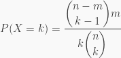
then in theory it would take
![\displaystyle E[X] = \frac{n+1}{m+1}.](https://s0.wp.com/latex.php?latex=%5Cdisplaystyle+E%5BX%5D+%3D+%5Cfrac%7Bn%2B1%7D%7Bm%2B1%7D.+&bg=f9f9f9&fg=333333&s=0&c=20201002)
I became interested in modeling this proposition so implemented a MATLAB program, try_keys(n,m), in which each key is represented by a number from 1 to n and each correct keys is represented by a number from 1 to m. And when the try_keys(n,m) is executed it outputs a random sequence that starts with any key and ends with a correct key.
Now in theory if had 15 keys, such that 3 keys are correct, then on average I would expect to open the door on the 4th try since

For Experiment1 I ran try_keys(15,3) a total of 10 times
try_keys(15,3)     =    13     7     4     6     5     1
try_keys(15,3)     =     4     2
try_keys(15,3)     =     3
try_keys(15,3)     =     4     5     1
try_keys(15,3)     =    14    10     5     4     2
try_keys(15,3)     =    12     4     3
try_keys(15,3)     =     7     1
try_keys(15,3)     =     2
try_keys(15,3)     =    15    10     6     1
try_keys(15,3)     =     4     9     1
and for Experiement2 I repeated the same thing
try_keys(15,3)     =    10     8     7     5     6     3
try_keys(15,3)     =    12     2
try_keys(15,3)     =    11     2
try_keys(15,3)     =     6     7     8     1
try_keys(15,3)     =    14     8     5     4     6     9     7    10     3
try_keys(15,3)     =     5     3
try_keys(15,3)     =    13     2
try_keys(15,3)     =     4     2
try_keys(15,3)     =     4     5    10     2
try_keys(15,3)     =    14    10     5     2
So from the first and second experiment, the average number of tries needed to open the door


are within 35% and 7.5% of

Now by the Law of large numbers we would expect that if we ran try_keys(15,3) an infinite number of times then the average would converge to 4. So, to illustrate this law I implemented average_try_keys(N,n,m) which runs try_keys(n,m), N times, and computes an average. And, I also implemented plot_average_try_keys(L,n,m) which plots average_try_keys(i*round(L/30),n,m) for integer values of i from 1 to 100. So, here are the plots that I got from plot_average_try_keys(L,15,3) using L values 1e2, 1e3, 1e4, 1e5 and 1e6.


And here is the code that I used to generate these plots.
try_keys
function [ s ] = try_keys(n,m)
%There are n keys which will be
%represented by numbers 1,2,...n.
%There are m correct keys which
%will be represented by numbers 1,2,...m.
%where m is less than or equal to n.
if( m > n || n <= 0 || m <= 0)
    bad_input = 1;
    quit;
end

%s is the sequence of keys draw will be s,
%where s(1) is the first key
%draw, s(2) the second, and so on.
%So at most we will try a total of n-m keys.
%s = zeros(1,n-m);
%We are assuming that that keys are
%uniformly distributed, so we will be
%using randi(10) but we wont be accepting
%keys which we have already
%tried.
s(1) = randi(n);

%We are done when we find a correct key so
%we check to see if first key is
%correct. If not then we get another key and so on.
if( size(find( s <= m ),2) ~= 0)
    done = 1;
else
    done = 0;
end
draw = 1;
while( done == 0)
isnewkey = 0;
while(isnewkey ==0)
    newkey = randi(n);
    if(size(find(s == newkey),2) == 0)
        s(draw + 1) = newkey;
        isnewkey = 1;
        if( size(find( s <= m ),2) ~= 0)
            done = 1;
        else
            draw = draw + 1;
        end
    end
end
end
end
average_try_keys
function mu = average_try_keys(N,n,m)
s =zeros(1,N);
for i=1:N
    s(i) =  size(try_keys(n,m),2);
end
mu = mean(s);
end
plot_average_try_keys
function plot_average_try_keys(L,n,m)
Num_points = 100;
expected_value = (n+1)/(m+1);
y = zeros(1,Num_points);
x = (1:Num_points)*round(L/Num_points);
for i=1:Num_points
y(i) = average_try_keys(i*round(L/Num_points),n,m);
end
plot(x,y,'-ro',x,expected_value,'-b')
h = legend('averages','expected value',2);
set(h,'Interpreter','none')
Random Keys
Posted: March 28, 2011 in examples, probabilityTags: binomial coefficient, expectation, fundamental counting principle, math, probability, probability mas function
Given 
First lest try to clarify the problem by picturing the following scenario. We have a bucket with 


So we are interested in calculating the expected value but first we need to derive a probability mass function which would tell us the probability of finding the correct key on the kth try, 
![\displaystyle E[X] = \sum_{k = 1}^{n-2}k P(X = k) .](https://s0.wp.com/latex.php?latex=%5Cdisplaystyle++E%5BX%5D+%3D+%5Csum_%7Bk+%3D+1%7D%5E%7Bn-2%7Dk+P%28X+%3D+k%29+.&bg=f9f9f9&fg=333333&s=0&c=20201002)
For 
P(finding correct key on 1st try)
which is given by

Since there are 3 correct keys then there are 3 ways in which the 1st choice could be a correct key. And, since there are

For 
P(finding correct key on 2nd try)
which can be thought of as
P(1st key was not correct and 2nd key is correct)
which is given by

Since there are 


If follows that

so in general
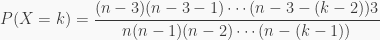
which can be simplified to

where the binomial coefficient 


So the average number of keys we would have to try, to find a correct key would be given by
![\displaystyle E[X] = \sum_{k=1}^{n-2} \frac{\displaystyle \binom{n-3}{k-1}3}{\displaystyle \binom{n}{k}}](https://s0.wp.com/latex.php?latex=%5Cdisplaystyle+E%5BX%5D+%3D+%5Csum_%7Bk%3D1%7D%5E%7Bn-2%7D+%5Cfrac%7B%5Cdisplaystyle+%5Cbinom%7Bn-3%7D%7Bk-1%7D3%7D%7B%5Cdisplaystyle+%5Cbinom%7Bn%7D%7Bk%7D%7D+&bg=f9f9f9&fg=333333&s=0&c=20201002)
which results in
![\displaystyle E[X] = \frac{n+1}{4}.](https://s0.wp.com/latex.php?latex=%5Cdisplaystyle+E%5BX%5D+%3D++%5Cfrac%7Bn%2B1%7D%7B4%7D.+&bg=f9f9f9&fg=333333&s=0&c=20201002)
